Surrogate keys have long played a vital role in the organization and management of data. It is, without a doubt, a pillar of dimensional modeling.  On May 2, 1998, the godfather (now grandfather) of dimensional modeling, Ralph Kimball, wrote:

[A] surrogate key in a data warehouse is more than just a substitute for a natural key. In a data warehouse, a surrogate key is a necessary generalization of the natural production key and is one of the basic elements of data warehouse design. Let’s be very clear: Every join between dimension tables and fact tables in a data warehouse environment should be based on surrogate keys, not natural keys. It is up to the data extract logic to systematically look up and replace^[a][b][c] every incoming natural key with a data warehouse surrogate key each time either a dimension record or a fact record is brought into the data warehouse environment.

I would argue that this “necessary generalization” doesn’t go far enough; it fails to emphasize the vital importance of the generalization, and abstraction, from the natural key, or any source artificial keys.  Case in point: in 2011, Netflix was pondering splitting off their DVD business, and there was internal discussion that the data and analytics would remain a centralized function of the overall organization.  On the surface, this made sense.  This would provide the organization with all their data in order to make the best predictions for their customers.  However, surrogates weren’t widely in use at the point of splitting the company (which, it should be noted, never happened), and now customers were going to be created by two separate organizations (or at the least, disparate systems), which meant that customer_id’s (integer values) were going inevitably going to be repeated, thereby combining people in the analytics environment who weren’t the same person, and skewing predictions terribly!  Alternatively, if surrogates had been applied within the analytics system, and abstracted away from the source systems, both source systems would have been able to generate independent customer_id’s with no impact to downstream systems.

There was no good excuse for not leveraging surrogate keys in traditional data warehouses.  It was a fundamental aspect and best practice of dimensional modeling, and generating surrogates was trivial, at best: (surrogate_key += 1).  Fast forward to the early days of Hadoop and easy-access to distributed systems, and the concept of surrogate keys was quickly disregarded, after a small handful of questionable attempts at continuing the best practice.

Where, oh where, did my surrogates go?

If surrogate keys are such a cornerstone to data warehousing dimensional modeling, did that somehow change when hadoop and distributed systems entered the mainstream?  Of course not.  Without wasting too much time re-hashing previous sins, it’s important to understand why it didn’t work, so we can we explain the nuances of how it still can.

First, look at the folks that made the initial foray into analytics in distributed systems: they were the data warehousing and ETL folks from the traditional RDBMS systems.  They (usually) recognized the value of surrogate keys, and they wanted to keep using them.  However, this is substantially more difficult in a distributed system, because each node (server/machine) in a cluster of servers/machines will naturally generate the same incremental values if they apply surrogate_key += 1 locally, and independently, of all other nodes in the cluster.  To put it simply, each individual node in a cluster will generate 1, 2, 3, …, so if you have four nodes in a cluster, you’ll generate four 1s, four 2s, four 3s, etc.  To be fair, if you know how many nodes are in your cluster, you can mathematically generate unique keys using various algorithms, such as the pseudo code below:

this_node_number + number_of_nodes * (previous_max_key += 1)

But one of the characteristics (benefits) of Hadoop is that the cluster is comprised of commodity hardware, so nodes can disappear, which means the number_of_nodes can change, but a purist will (correctly) argue that it doesn’t matter: gaps in surrogate keys are perfectly fine.  In fact, there should be no “intelligence” to a surrogate.  That is correct, but another of the benefits of Hadoop is that just as nodes can disappear (scaling in, or a loss of nodes due to hardware failures), the cluster size can be increased (scaling out) when more nodes are added.  It is the latter situation where the problem arises, as the aforementioned algorithm(s) will begin to generate duplicates.  

What was the next solution?  Simply generate the surrogates on a single node, and go back to using the comfortable algorithm: surrogate_key += 1.  Problem solved.  Except, we’ve completely undone the value of distributed systems by running things serially!  This means that while we adopted Hadoop (at least in part) to increase volumes and velocity (hooray for big data and the systems that enable them!), we decided to forego the benefits in order to retain surrogate keys.  It is easy to see what would inevitably eventually occur: forget surrogate keys completely.  Just use the natural keys, and disregard the previous advice and fundamental rule of “[e]very join between dimension tables and fact tables in a data warehouse environment should be based on surrogate keys, not natural keys”.

So we love surrogates just like we always did, but we found out that they’re hard to do in distributed systems, at least without throwing away all the power of horizontal scalability, so it seems that the trade-off is: the performance of distributed systems vs the value that surrogate keys provide.  It is the culmination of seemingly small concessions, like this, that led the traditional data warehouse to become the re-branded data lake, which inevitably (always) eventually leads to the dreaded data swamp.

Solution

Now that we’ve (hopefully!) sufficiently explained why we’ve always loved surrogates, and continue to, and how we got to the place where we’ve disregarded them when moving to distributed systems, let’s turn our attention to implementing a solution that provides us the benefits of surrogates, without foregoing the benefits of distributed systems.

It’s time to put the discipline into distributed data warehousing

Let’s look at one of the overlooked attributes of a traditional surrogate: the data type.  Per Wikipedia, “[s]urrogate keys tend to be a compact data type, such as a four-byte integer”.  Why?  Mostly, it’s about space, and in traditional RDBMS data warehouses, space was of the essence.  One of the major factors that led to the creation and open sourcing of Hadoop, and distributed systems based on commodity hardware, is the massive drop in cost of storage, as illustrated below:

Disk (storage) is no longer a concern, or at the very least, that concern has changed dramatically, but for some reason, we data warehousing and analytics practitioners have a bad habit of continuing to consider to think of surrogates as synonymous with integers.  The reality is that surrogates are supposed to accomplish the primary concerns of:

• Allowing the database to query the single key column faster than it could multiple columns
• Surrogate keys are also less expensive to join (fewer columns to compare) than compound keys
• The benefit of abstraction, as described previously in this document

If we’re free from the shackles of limited space, which is further amplified by the use of cloud resources, there is nothing about accomplishing those objectives that have anything to do with data types.

Modern surrogate data types

Instead of the compact, space-saving integer surrogates, in our non-restrictive distributed system, use UUIDs.  While not as compact as integers, this addresses multiple challenges, such as not needing to apply keys serially (the surrogate_key += 1 approach), because UUIDs can applied easily, and in parallel (distributed), using simple code such as:

#!/usr/bin/python

import uuid

surrogate = str(uuid.uuid4())

Each call to uuid generates a unique value, or at a minimum, with only a minute chance of collision:

• [T]he number of random version 4 UUIDs which need to be generated in order to have a 50% probability of at least one collision is 2.71 quintillion
• This number is equivalent to generating 1 billion UUIDs per second for about 85 years, and a file containing this many UUIDs, at 16 bytes per UUID, would be about 45 exabytes, many times larger than the largest databases currently in existence, which are on the order of hundreds of petabytes

When do we generate a new uuid?

The same way we always did: when we see a new natural key.  The natural key, as explained by Wikipedia, is as follows:

A natural key (also known as business key) is a type of unique key, found in relational model database design, that is formed of attributes that already exist in the real world. It is used in business-related columns. In other words, a natural key is a candidate key that has a logical relationship to the attributes within that row.^[d]

In practice

What does this look like in practice?  Imagine the following set of customer data:

Before going forward, let’s make one distinction: the cust_id is not part of the natural key.  It is an artificial key that was generated upstream from the data platform.  Reflecting back to the Netflix example provided earlier, it’s beyond the control of the data platform to dictate what the source systems might do (or have to do), and as such we must not rely on it.  Instead, we want to generate our own key (our UUID surrogate), and rely on the natural key (or potentially the natural key + the artificial keys) to determine when a new surrogate is required.^[e]

Hashing

One well-known pattern for determining if an incoming record is new is to hash the natural key, which makes comparing new and existing rows easier, based on the earlier principal of single keys being “less expensive to join (fewer columns to compare) than compound keys”.  In the above example, the natural key of the table is (probably)^[f] [fname, lname].  We can add a hash value to each row, using the following simple script:

import hashlib

hashlib.md5(fname+lname).hexdigest()

This results in the table being extended a single column, as shown below:

As each row in the above table contains a unique hash key, each would generate a new (UUID) surrogate, which has been appended below:

Now, when new data arrives:

We follow the same procedure: hash the natural key, compare against existing.  If the hash key exists, re-use the surrogate.  If not, generate a new one:

Changing natural keys

We’d be remiss if we didn’t discuss evolving natural keys, as this is a very common scenario in real-world applications.  For the sake of simplicity in illustration, imagine that the data set we’ve used throughout this paper is extended to include gender, which becomes part of the new natural key:

This changes the hash values, as indicated below:

In this case, if we were to join the existing row:

Maggie O’Connell (c673e6fef25d50a3ffec15cee1c31c27)

to the new hash for the same original row:

Maggie O’Connell F[emale] (0ae1d64c6e85ea7bda7810a785ca262b)

we’d find a difference, and a new UUID would incorrectly be generated.

The impact of immutable disk

Remember that we’re talking here specifically about (Hadoop) distributed systems, and these systems include immutable storage systems (e.g. HDFS, S3).  This characteristic dictates certain changes in data modeling that go beyond minor nuances like whether surrogates need be integers or strings.  They also dictate that data should be pre-joined to avoid shuffling in the consumption layer, as well as other nuances, most of which beyond the scope of this document.  However, because of the impact on surrogate keys, it is necessary to quickly discuss one nuanced modeling approach in distributed systems with immutable disk: full dimension restatement.

Full dimension restatement

We sometimes refer to the _DAY_D pattern with regard to dimensional modeling in distributed systems with immutable storage.  In short, it says the ETL pattern of dimensions (not facts) should follow the pattern of:

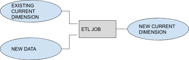
In which the entirety of the current existing dimension is (full outer) joined to newly arriving data, and the complete dimension is re-stated.  It is sometimes referred to as the _DAY_D pattern because oftentimes the data is restated like this once daily.

What it results in is a single partition per day, which contains the entire dimension volume, as shown below:

...

s3://my-bucket/my_database.db/customer/as_of_date=2017-09-26

s3://my-bucket/my_database.db/customer/as_of_date=2017-09-27

s3://my-bucket/my_database.db/customer/as_of_date=2017-09-28

…

And so on.  Obviously, querying all partitions will result in double counting of any customers that existed as-of September 26th (or earlier).  Thus, another unpartitioned table DDL simply points to the most recent S3 location (in the above example), and voilà, you have a CUSTOMER_CURRENT table without the risk of double-counting (no duplicates), and without having to do any additional data processing.

This gives you the benefit of slowly changing dimensions (reading data across the as_of_date partitions) as well as the safety of a single customer dimension reflecting the current state of what-you-know about your customers (the *_CURRENT table), without having to re-state the data to disk again.  With distributed systems, this approach can scale to the hundreds of millions, which will accommodate the vast majority of (properly modeled) dimensional data.

When it comes to transactional (measurement) data, or traditional facts, it’s not reasonable to re-state data regularly.  While we may have “only” 10,000,000 customers, those customers may have billions or trillions of transactions.  We want to rely on single key joins (thank you, surrogates), but we can’t make those joins the hash, because the hashes change (damn you, evolving natural keys).

The rule of thumb, then, is this:

Restate your dimensions in full, with a primary partition key reflecting the cadence in which you execute. Append facts, and partition them by the transaction date.  The dimensions contain as-of hashes and (consistent) uuid surrogates, and the facts contain only the (consistent) surrogates.

Now I’m confused.  How does this apply to surrogate keys?

This applies to surrogate keys because we generate surrogates using hashes, and we know that the natural key changes over time, which means the hashes change over time, which means we’ll have to re-state the dimension every time the natural key changes, but we’re already re-stating the dimensions in full anyway to follow our data modeling best practice, so we don’t have to worry about natural key evolution.  It’s business-as-usual, with only an additional execution to re-state the hashes on the dimension:

Before restatement:

After re-statement, because of natural key evolution, or as part of a normal full re-statement execution:

As you can see, the hash has changed, but the surrogate remains static.  This allows the (*_CURRENT) dimension to continuously reflect the accurate hash_key, while always reflecting a continuous surrogate key.  It further allows for transactional/fact data to not require re-stating (append only), and to house a single key for join optimization (performance/ease of use).  

For the sake of illustration, a fact table is shown below with a hash key appended to the table, so that we can see how the hash changes over time, but the surrogate remains static.  Noting again that the hash would not actually be included on the dimension because it is not consistent over time: